Sample Normal Distribution

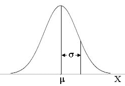
This is the weighted center of the distribution, meaning that it is highly susceptible to the influence of skewness and outliers. In this simulation, we assume a normal distribution but in a non-normal distribution, the median is usually a better indication of center. Please use the keyboard to enter numbers with more than two significant digits.

This is the spread of the sample. A greater standard deviation is indicative of a wider distribution, however, this will not affect normality. Similar to the mean, standard deviation is an easily influenced measure of spread. In a non-normal distribution, the inter-quartile-range and quartiles are better indicators of spread.

This is the number of simulations that will be performed. For each simulation, the sample mean, $\overline x $, will be calculated in the standard method by summing the elements of the sample and then dividing by the total size of the sample, i.e. $\frac{1}{n}\sum\limits_{i = 1}^n {{x_i}} $.

This is the size of the simulated sample or how many random x‘s we are drawing in each sample. The larger the sample size is, the closer samples should follow the population distribution, which in this case is normal (bell-curve shaped) since the influence of outliers is diminished.

This will not affect calculations in any way. Output data will be reported to this number of digits after rounding. Two decimal places is typical. The distribution of sample proportions can be easily plotted in a dot plot or histogram.